Spatial Analysis of Gene Diversity

Estimate spatial gene diversity (expected heterozygozity - He) through the individual-centred approach by Manel et al. (2007). sHe() calculates the unbiased estimate of He based on the information of allele frequency obtained from codominant or dominant markers in individuals within a circular moving windows of known radius over the sampling area.

sHe(x, coord.cols = 1:2, marker.cols = 3:4, 
  marker.type = c("codominant", "dominant"), 
  grid = NULL, latlong2km = TRUE, radius, nmin = NULL)

Arguments

x	a data frame or numeric matrix containing columns with coordinates of individuals and marker genotyping
coord.cols	a vector of integer giving the columns of coordinates in `x`
marker.cols	a vector of integer giving the columns of markers in `x`
marker.type	a character; the type of molecular marker
grid	optional; a two-column matrix containing coordinates over which to predict He
latlong2km	logical; should coordinates be converted from lat/long format into kilometer-grid based?
radius	the radius of the moving window. It must be in the same format as sampling coordinates
nmin	optional; a numeric value indicating the minimum number of individuals used to calculate He. If is the number of individuals in a certain location is less then `nmin`, `sHe` will consider He as zero.

Details

The unbiased estimate of expected heterogygozity (Nei, 1978) is given by:

$$ He = (1 - \sum_{i=1}^{n} p_{i}^{2}) \frac{2n}{2n - 1} $$

where $p_{i}$ is the frequency of the i-th allele per locus considering the $n$ individuals in a certain location.

Value

A list of

diversity

a data frame with the following columns: coord.x - the x-axis coordinates of the predicion grid, coord.y - the y-axis coordinates of the predicion grid, n - the number of individuals in a certain points in the grid, MaxDist - the maximum observed distance among these individuals, uHe - the unbiased estimate of gene diversity (as expressed above), and SE - the standard error of uHe.

mHe

a matrix containing the estimates of He for every marker, on each point of the grid.

locations

a numeric matrix containing the sampling coordinates, as provides as input.

References

da Silva, A.R.; Malafaia, G.; Menezes, I.P.P. (2017) biotools: an R function to predict spatial gene diversity via an individual-based approach. Genetics and Molecular Research, 16: gmr16029655.

Manel, S., Berthoud, F., Bellemain, E., Gaudeul, M., Luikart, G., Swenson, J.E., Waits, L.P., Taberlet, P.; Intrabiodiv Consortium. (2007) A new individual-based spatial approach for identifying genetic discontinuities in natural populations. Molecular Ecology, 16:2031-2043.

Nei, M. (1978) Estimation of average heterozygozity and genetic distance from a small number of individuals. Genetics, 89: 583-590.

Author

Anderson Rodrigo da Silva <anderson.agro@hotmail.com>

Ivandilson Pessoa Pinto de Menezes <ivan.menezes@ifgoiano.edu.br>

Warning

Depending on the dimension of x and/or grid, sHe() can be time demanding.

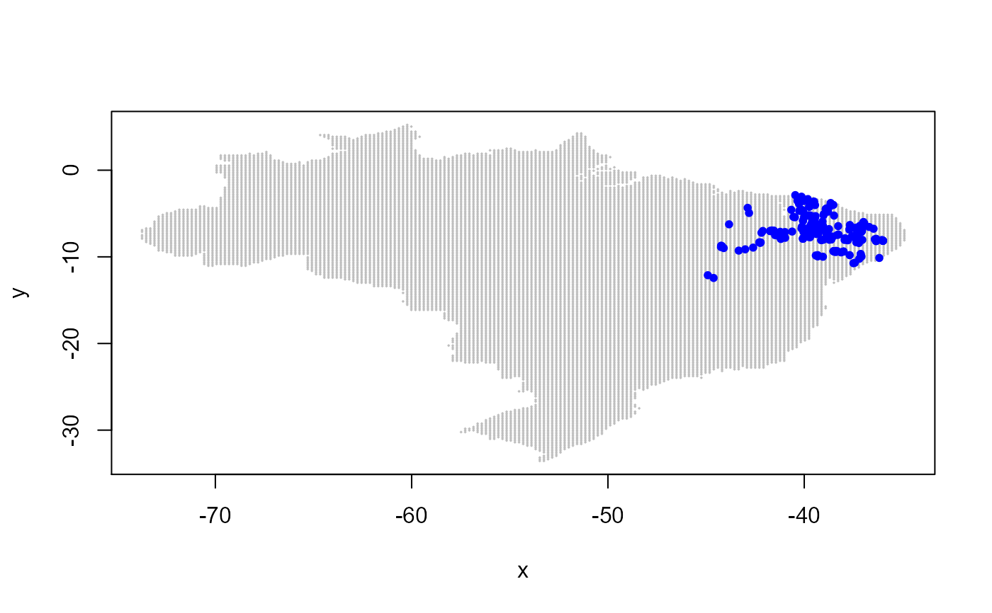
Examples

data(moco)
data(brazil)

# check points
plot(brazil, cex = 0.1, col = "gray")
points(Lat ~ Lon, data = moco, col = "blue", pch = 20)

# using a retangular grid (not passed as input!)
# ex <- sHe(x = moco, coord.cols = 1:2,
#  marker.cols = 3:20, marker.type = "codominant",
#  grid = NULL, radius = 150)
#ex
# plot(ex, xlab = "Lon", ylab = "Lat")

# A FANCIER PLOT...
# using Brazil's coordinates as prediction grid
# ex2 <- sHe(x = moco, coord.cols = 1:2,
#  marker.cols = 3:20, marker.type = "codominant",
#  grid = brazil, radius = 150)
# ex2
#
# library(maps)
# borders <- data.frame(x = map("world", "brazil")$x, 
#  y = map("world", "brazil")$y)
#
# library(latticeExtra)
# plot(ex2, xlab = "Lon", ylab = "Lat", 
#  xlim = c(-75, -30), ylim = c(-35, 10), aspect = "iso") +
#   latticeExtra::as.layer(xyplot(y ~ x, data = borders, type = "l")) +
#   latticeExtra::as.layer(xyplot(Lat ~ Lon, data = moco))

# End (not run)