About
In this package you will find a series of functions for soil physics data analysis. These functions includes five models of water retention curve, seven methods of soil precompression stress, least limiting water range (LLWR), Integral Water Capacity (IWC), soil penetration resistance curve by Busscher’s model, calculation of Soil Aggregate-Size Distribution, S Index, critical soil moisture and maximum bulk density using data from Proctor test, calculation of equivalent pore radius as a function of soil water tension, simulation of sedimentation time of soil particles through Stokes’ law, simulation of soil pore size distribution, calculation of the hydraulic cut-off introduced by Dexter et al. (2008) and simulation of soil compaction induced by agricultural field traffic. Other utilities like functions to calculate the void ratio and to determine the maximum curvature point are also available.
Instalation
You can install and load the released version of soilphysics from GitHub with:
install.packages("devtools")

devtools::install_github("arsilva87/soilphysics")

library(soilphysics)
Soil compaction tools
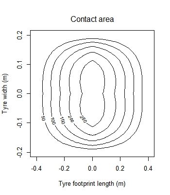
Using the function stressTraffic, it it possible calculate the contact area, stress distribuition and stress propagation based on the SoilFlex model.
# Usage
stress <- stressTraffic(inflation.pressure=200,
	   recommended.pressure=200,
	   tyre.diameter=1.8,
	   tyre.width=0.4,
	   wheel.load=4000,
	   conc.factor=c(4,5,5,5,5,5),
           layers=c(0.05,0.1,0.3,0.5,0.7,1),
	   plot.contact.area = TRUE)

# Results
 ---------- Boundaries of Contact Area

    Parameters  Value Units
1   Max Stress 289.00 kPa
2 Contact Area   0.29 m^2
3  Area Length   0.83  m
4   Area Width   0.40  m

 ---------- Wheel Loads

          Parameters Loads (kg)
1 Applied Wheel Load       4000
2 Modeled Wheel Load       4030
3          Diference        -30

 ---------- Stress Propagation

  Layers (m) Zstress   p
1       0.05     275 169
2       0.10     262 132
3       0.30     154  62
4       0.50      85  31
5       0.70      51  18
6       1.00      28  10
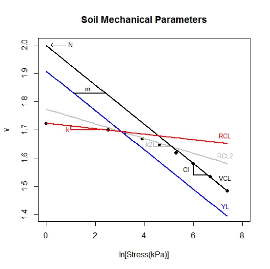
Unsing the funtion soilDeformation, it is possible calculates the bulk density variation as a function of the applied mean normal stress using critical state theory, by O’Sullivan and Robertson (1996).
# Usage
soilDeformation(stress = 300,
                p.density = 2.67,
	        iBD = 1.55,
                N = 1.9392,
                CI = 0.06037,
                k = 0.00608,
                k2 = 0.01916,
                m = 1.3,graph=TRUE,ylim=c(1.4,2.0))

# Results
   iBD    fBD     vi     vf   I%
1 1.55 1.6385 1.7226 1.6295 5.71
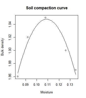
Critical soil moisture and maximum bulk density (Proctor test)
mois <- c(0.083, 0.092, 0.108, 0.126, 0.135)
bulk <- c(1.86, 1.92, 1.95, 1.90, 1.87)

# Usage
criticalmoisture(theta = mois, Bd = bulk)

# Results
          Critical Moisture and Maximum Bulk Density

                  Sample 1
Intercept        0.4825950
mois            26.9265767
mois^2        -123.7120431
R.squared        0.9515476
n                5.0000000
critical.mois    0.1088276
max.bulk         1.9477727
Soil water availability tools
Quantifying the soil water availability for plants through the IWC approach:
# Usage
iwc(theta_R = 0.166, theta_S = 0.569, alpha = 0.029, n = 1.308,
    a = 0.203, b = 0.256, hos = 200, graph = TRUE)

# Results
                     IWC       EI         h.Range
EKa(h, hos)    0.0144000   0.9600  66.43 - 139.49
EK(h, hos)     0.0405000   5.3700    139.49 - 330
C(h, hos)      0.0846000  49.4800   330 - 2471.44
ER(h, hos)     0.0288000  87.1200 2471.44 - 15000
ERKdry(h, hos) 0.0006000   4.9100   12000 - 15000
Sum            0.1689139 147.8336       0 - 15000
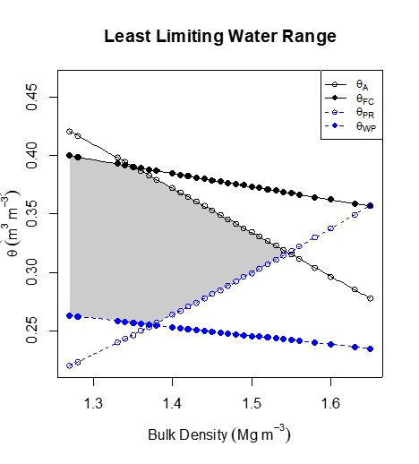
Quantifying the soil water availability for plants through the LLWR approach:
# Usage
data(skp1994)
ex1 <- with(skp1994,
	 llwr(theta = W, h = h, Bd = BD, Pr = PR,
		particle.density = 2.65, air = 0.1,
		critical.PR = 2, h.FC = 100, h.WP = 15000))

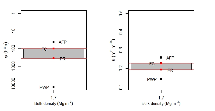
Quantifying the LLWR using van Genuchten’s parameters:
# Usage
  par(mfrow=c(1,2))
  llwr_llmpr(thetaR=0.1180, thetaS=0.36, alpha=0.133, n=1.30,
        d=0.005, e=-2.93, f=3.54, PD=2.65,
        critical.PR=4, h.FC=100, h.PWP=15000, air.porosity=0.1,
        labels=c("AFP", "FC","PWP", "PR"),
        graph1=TRUE,graph2=FALSE, ylab=expression(LLMPR~(hPa)), ylim=c(15000,1))
  mtext(expression("Bulk density"~(Mg~m^-3)),1,line=2.2, cex=0.8)

  llwr_llmpr(thetaR=0.1180, thetaS=0.36, alpha=0.133, n=1.30,
        d=0.005, e=-2.93, f=3.54, PD=2.65,
        critical.PR=4, h.FC=100, h.PWP=15000, air.porosity=0.1,
        labels=c("AFP", "FC","PWP", "PR"),
        graph1=FALSE,graph2=TRUE, ylab=expression(LLMPR~(hPa)), ylim=c(0.1,0.5))
  mtext(expression("Bulk density"~(Mg~m^-3)),1,line=2.2, cex=0.8)

# Results
$CRITICAL_LIMITS
     theta potential
AIR 0.2600     41.02
FC  0.2285    100.00
PWP 0.1428  15000.00
PR  0.1939    356.65

$LLRW_LLMPR
         Upper    Lower    Range
LLWR    0.2285   0.1939   0.0346
LLMPR 100.0000 356.6500 256.6500
Precompression stress
Estimating the precompression stress by several methods:

pres <- c(1, 12.5, 25, 50, 100, 200, 400, 800, 1600)
VR <- c(0.846, 0.829, 0.820, 0.802, 0.767, 0.717, 0.660, 0.595, 0.532)

# Usage
sigmaP(VR, pres, method = "casagrande", n4VCL = 2)

# Results
Preconsolidation stress: 104.2536
Method: casagrande, with mcp equal to 1.7885
Compression index: 0.2093
Swelling index: 0.0179
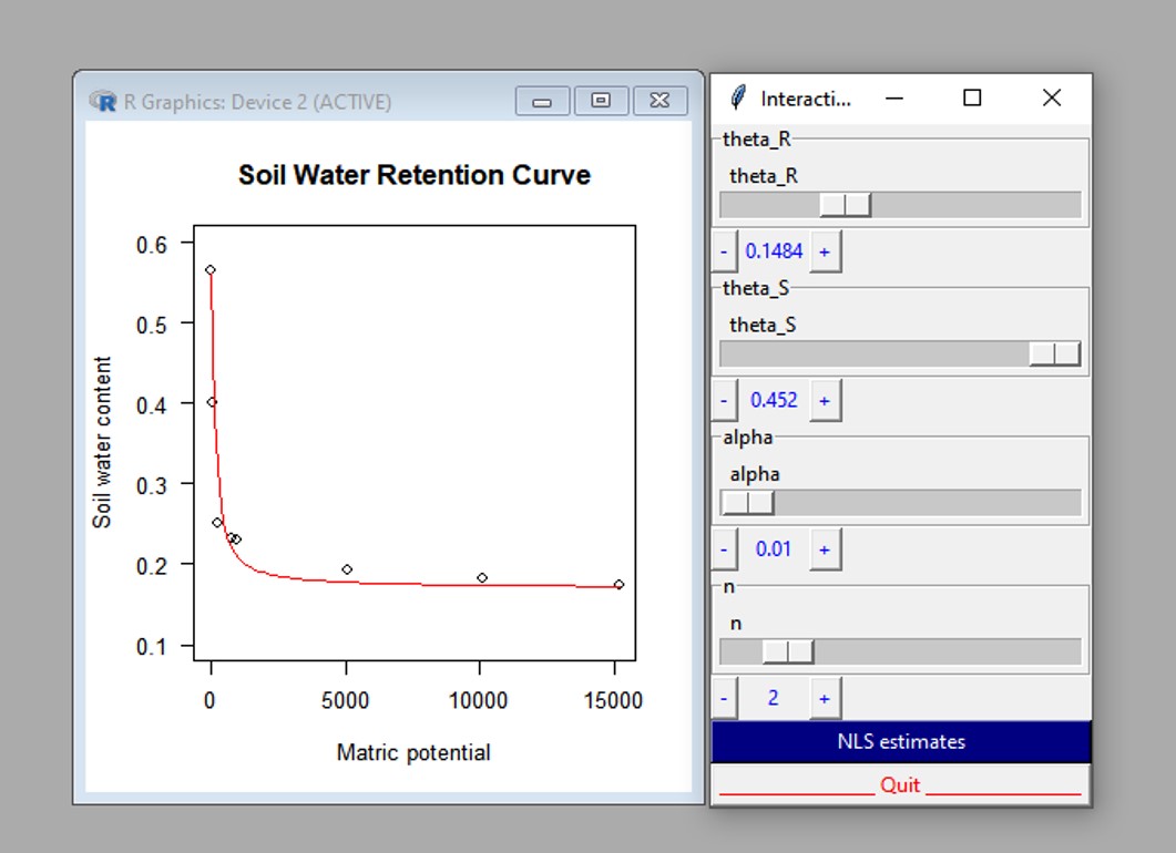
Soil water retention curve
Fitting water retention curve using van Genuchten’s model
h <- c(0.001, 50.65, 293.77, 790.14, 992.74, 5065, 10130, 15195)
w <- c(0.5650, 0.4013, 0.2502, 0.2324, 0.2307, 0.1926, 0.1812, 0.1730)

# Usage
fitsoilwater(theta=w, x=h, ylim=c(0.1,0.6))

# Results
Parameters:
        Estimate Std. Error t value Pr(>|t|)
theta_R  0.16761    0.01272  13.179 0.000192 ***
theta_S  0.56531    0.01092  51.786 8.32e-07 ***
alpha    0.04748    0.01177   4.035 0.015671 *
n        1.52926    0.09579  15.965 9.00e-05 ***
---
S Index
# Usage
Sindex(theta_R=0, theta_S=0.395, alpha=0.0217,
       n=1.103)

# Results
          The S Index

h_i : 395.4757
theta_i : 0.3139
|S| : 0.0296
Soil physical quality : Poor
Soil Aggregate-Size Distribution
data(SoilAggregate)
head(SoilAggregate)
  ID    D3 D1.5 D0.75 D0.375 D0.178 D0.053
1 A1 25.80 7.55  5.50   5.10   3.00   3.05
2 A2 19.85 5.30  7.45   7.30   4.40   5.70
3 A3  7.10 9.80 11.60   8.10   2.35  11.05
4 B1  6.10 4.85 11.20  13.10   7.15   7.60
5 B2 12.00 6.30 16.10   7.35   3.70   4.55
6 B3 14.10 6.15  8.80  11.05   4.60   5.30

classes <- c(3, 1.5, 0.75, 0.375, 0.178, 0.053)

# Usage
out <- aggreg.stability(sample.id = SoilAggregate[ ,1],
                        dm.classes = classes,
                        aggre.mass = SoilAggregate[ ,-1])


# Results
head(out)
  sample.id      MWD       GMD total.mass X3 X1.5 X0.75 X0.375 X0.178 X0.053
1        A1 1.909163 1.2382214         50 52   15    11     10      6      6
2        A2 1.538206 0.8239103         50 40   11    15     15      9     11
3        A3 0.974829 0.4865272         50 14   20    23     16      5     22
4        B1 0.811260 0.4311214         50 12   10    22     26     14     15
5        B2 1.223620 0.7282644         50 24   13    32     15      7      9
6        B3 1.267369 0.6853162         50 28   12    18     22      9     11
Spin-off
Sedimentation time of soil particle (Stokes’ law): https://renatoagro.shinyapps.io/stokesapp/
Exploring water retention curve using van Genuchten’s model: https://soilphysics.shinyapps.io/wrcAPP/
Soil Aggregate-Size Distribution: https://renatoagro.shinyapps.io/Agre/
Usual Least Limiting Water Range (LLWR): https://soilphysics.shinyapps.io/LLWRAPP/
Water suction at the point of hydraulic cut-off (Dexter et al. 2012): https://soilphysics.shinyapps.io/h_cutoff/
LLWR and LLMPR: https://soilphysics.shinyapps.io/LLWR_LLMPR/
PredComp 1.0: https://appsoilphysics.shinyapps.io/PredComp/
fisoilwater: https://appsoilphysics.shinyapps.io/fitsoilwaterAPP/
Automatically fit the Water Retention Curve online: ![]()
Citation and references
De Lima, R.P.; Tormena, C.A.; Figueiredo, G.C; Da Silva, A.R.; Rolim, M.M. (2020) Least limiting water and matric potential ranges of agricultural soils with calculated physical restriction thresholds. Agricultural Water Management, 240: 106299. DOI: https://doi.org/10.1016/j.agwat.2020.106299
Da Silva, A.R.; De Lima, R.P. (2017) Determination of maximum curvature point with the R package soilphysics. International Journal of Current Research, 9: 45241-45245.
De Lima, R.P.; Da Silva, A.R.; Da Silva, A.P.; Leao, T.P.; Mosaddeghi, M.R. (2016) soilphysics: an R package for calculating soil water availability to plants by different soil physical indices. Computers and Eletronics in Agriculture, 120: 63-71. DOI: https://doi.org/10.1016/j.compag.2015.11.003
Da Silva, A.R.; De Lima, R.P. (2015) soilphysics: an R package to determine soil preconsolidation pressure. Computers and Geosciences, 84: 54-60. DOI: https://doi.org/10.1016/j.cageo.2015.08.008
Contributions and bug reports
soilphysics is an ongoing project. Then, contributions are very welcome. If you have a question or have found a bug, please open an Issue or reach out directly by e-mail: anderson.silva@ifgoiano.edu.br or renato_agro_@hotmail.com.
By
Anderson R. da Silva & Renato P. de Lima