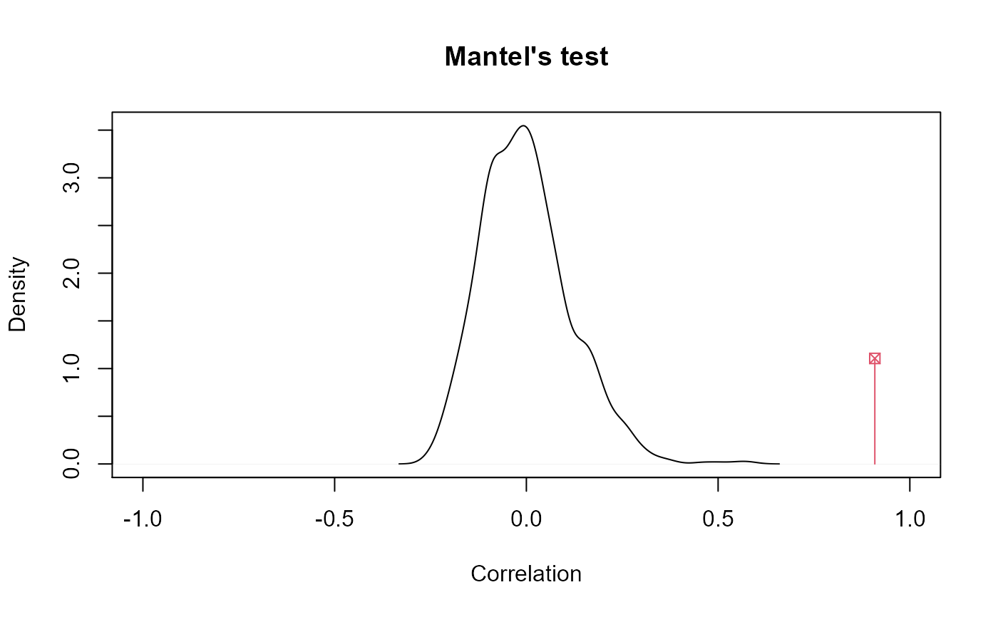
Mantel's Permutation Test
mantelTest.RdMantel's permutation test based on Pearson's correlation coefficient to evaluate the association between two distance square matrices.
mantelTest(m1, m2, nperm = 999, alternative = "greater",
  graph = TRUE, main = "Mantel's test", xlab = "Correlation", ...)
Arguments
| m1 | an object of class "matrix" or "dist", containing distances among n individuals. |
|---|---|
| m2 | an object of class "matrix" or "dist", containing distances among n individuals. |
| nperm | the number of matrix permutations. |
| alternative | a character specifying the alternative hypothesis. It must be one of "greater" (default), "two.sided" or "less". |
| graph | logical; if TRUE (default), the empirical distribution is plotted. |
| main | opitional; a character describing the title of the graphic. |
| xlab | opitional; a character describing the x-axis label. |
| ... | further graphical arguments. See |
Value
A list of
numeric; the observed Pearson's correlation between m1 and m2.
numeric; the empirical p-value of the permutation test.
character; the alternative hypothesis used to compute p.value.
numeric vector containing randomized values of correlation, i.e., under the null hypothesis that the true correlation is equal to zero.
References
Mantel, N. (1967). The detection of disease clustering and a generalized regression approach. Cancer Research, 27:209--220.
Author
Anderson Rodrigo da Silva <anderson.agro@hotmail.com>
See also
Examples
#> 1 2 3 4 5 6 7 #> 2 3.340628 #> 3 4.077546 5.506977 #> 4 5.363563 1.998527 4.850491 #> 5 3.101330 5.045423 2.324152 8.089021 #> 6 1.238522 2.651805 4.679259 4.811098 4.688428 #> 7 3.623305 1.724090 7.135583 2.134167 8.605810 1.934920 #> 8 2.922838 1.690728 6.582117 1.663528 6.833739 3.374794 2.111143 #> 9 3.555213 1.788716 7.199125 1.423100 8.037689 4.189185 2.353159 #> 10 5.446132 1.208638 5.884702 0.795171 7.918028 4.029226 1.048315 #> 11 7.978329 2.567743 5.938755 2.178913 7.412238 6.105662 3.410709 #> 12 5.840065 1.294550 7.029946 0.694369 8.241306 5.737707 2.587998 #> 13 8.453048 2.406380 9.802441 3.373966 8.923391 8.698328 4.615716 #> 14 1.465736 4.031444 5.534711 7.206169 2.856060 3.086537 4.635934 #> 15 2.396303 2.164605 8.414811 3.583914 7.753116 2.968316 1.327477 #> 16 2.690305 7.437900 4.709341 9.946683 3.378140 5.786071 8.758748 #> 17 3.134917 4.103622 7.657465 3.619184 9.311149 3.947882 1.866983 #> 8 9 10 11 12 13 14 #> 2 #> 3 #> 4 #> 5 #> 6 #> 7 #> 8 #> 9 0.222560 #> 10 2.378080 2.396474 #> 11 4.203915 4.887162 1.142472 #> 12 1.166367 0.940243 1.019113 2.206098 #> 13 3.830709 3.863815 2.128390 2.317785 1.503503 #> 14 4.862576 5.862818 5.754145 7.306173 6.872372 6.610267 #> 15 1.693882 1.815781 2.678664 5.821163 2.968784 4.095387 2.594153 #> 16 8.813287 9.189764 9.518194 12.176680 10.766776 11.399043 1.953576 #> 17 3.241800 3.066397 3.199140 7.043761 4.326943 6.149939 3.599164 #> 15 16 #> 2 #> 3 #> 4 #> 5 #> 6 #> 7 #> 8 #> 9 #> 10 #> 11 #> 12 #> 13 #> 14 #> 15 #> 16 6.103552 #> 17 0.942114 5.441962#> #> Tocher's Clustering #> #> Call: tocher.dist(d = garlicdist) #> #> Cluster algorithm: original #> Number of objects: 17 #> Number of clusters: 6 #> Most contrasting clusters: cluster 3 and cluster 5, with #> average intercluster distance: 11.78786 #> #> $`cluster 1` #> [1] 8 9 12 4 10 2 7 15 #> #> $`cluster 2` #> [1] 1 6 14 #> #> $`cluster 3` #> [1] 11 13 #> #> $`cluster 4` #> [1] 3 5 #> #> $`cluster 5` #> [1] 16 #> #> $`cluster 6` #> [1] 17 #>#> 1 2 3 4 5 6 7 #> 2 4.333530 #> 3 4.156222 7.070493 #> 4 4.333530 1.745434 7.070493 #> 5 4.156222 7.070493 2.324152 7.070493 #> 6 1.930265 4.333530 4.156222 4.333530 4.156222 #> 7 4.333530 1.745434 7.070493 1.745434 7.070493 4.333530 #> 8 4.333530 1.745434 7.070493 1.745434 7.070493 4.333530 1.745434 #> 9 4.333530 1.745434 7.070493 1.745434 7.070493 4.333530 1.745434 #> 10 4.333530 1.745434 7.070493 1.745434 7.070493 4.333530 1.745434 #> 11 7.525301 3.264753 8.019206 3.264753 8.019206 7.525301 3.264753 #> 12 4.333530 1.745434 7.070493 1.745434 7.070493 4.333530 1.745434 #> 13 7.525301 3.264753 8.019206 3.264753 8.019206 7.525301 3.264753 #> 14 1.930265 4.333530 4.156222 4.333530 4.156222 1.930265 4.333530 #> 15 4.333530 1.745434 7.070493 1.745434 7.070493 4.333530 1.745434 #> 16 3.476651 8.816863 4.043741 8.816863 4.043741 3.476651 8.816863 #> 17 3.560654 3.045773 8.484307 3.045773 8.484307 3.560654 3.045773 #> 8 9 10 11 12 13 14 #> 2 #> 3 #> 4 #> 5 #> 6 #> 7 #> 8 #> 9 1.745434 #> 10 1.745434 1.745434 #> 11 3.264753 3.264753 3.264753 #> 12 1.745434 1.745434 1.745434 3.264753 #> 13 3.264753 3.264753 3.264753 2.317785 3.264753 #> 14 4.333530 4.333530 4.333530 7.525301 4.333530 7.525301 #> 15 1.745434 1.745434 1.745434 3.264753 1.745434 3.264753 4.333530 #> 16 8.816863 8.816863 8.816863 11.787861 8.816863 11.787861 3.476651 #> 17 3.045773 3.045773 3.045773 6.596850 3.045773 6.596850 3.560654 #> 15 16 #> 2 #> 3 #> 4 #> 5 #> 6 #> 7 #> 8 #> 9 #> 10 #> 11 #> 12 #> 13 #> 14 #> 15 #> 16 8.816863 #> 17 3.045773 5.441962#> #> Mantel's permutation test #> #> Correlation: 0.9086886 #> p-value: 0.001, based on 999 matrix permutations #> Alternative hypothesis: true correlation is greater than 0# End (Not run)